
Note
Go to the end to download the full example code.
Tutorial on learning N-MNIST classification with e-prop
Run this example as a Jupyter notebook:

See our guide for more information and troubleshooting.
Training a classification model using supervised e-prop plasticity to classify the Neuromorphic MNIST (N-MNIST) dataset.
Description
This script demonstrates supervised learning of a classification task with the eligibility propagation (e-prop) plasticity mechanism by Bellec et al. [1] with additional biological features described in [3].
The primary objective of this task is to classify the N-MNIST dataset [2], an adaptation of the traditional MNIST dataset of handwritten digits specifically designed for neuromorphic computing. The N-MNIST dataset captures changes in pixel intensity through a dynamic vision sensor, converting static images into sequences of binary events, which we interpret as spike trains. This conversion closely emulates biological neural processing, making it a fitting challenge for an e-prop-equipped spiking neural network (SNN).
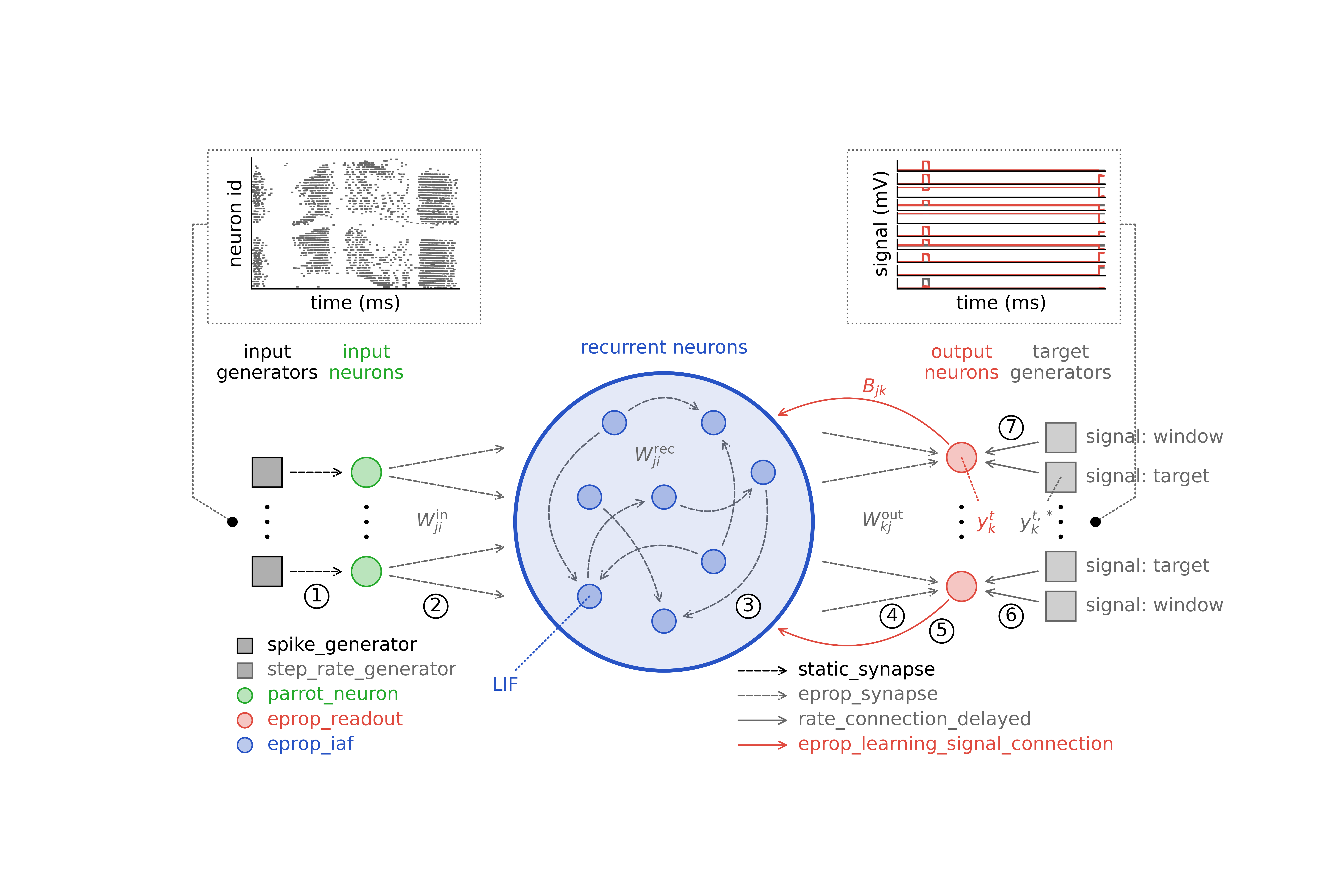
Learning in the neural network model is achieved by optimizing the connection weights with e-prop plasticity. This plasticity rule requires a specific network architecture depicted in Figure 1. The neural network model consists of a recurrent network that receives input from spike generators and projects onto multiple readout neurons - one for each class. Each input generator is assigned to a pixel of the input image; when an event is detected in a pixel at time \(t\), the corresponding input generator (connected to an input neuron) emits a spike at that time. Each readout neuron compares the network signal \(y_k\) with the teacher signal \(y_k^*\), which it receives from a rate generator representing the respective digit class. Unlike conventional neural network classifiers that may employ softmax functions and cross-entropy loss for classification, this network model utilizes a mean-squared error loss to evaluate the training error and perform digit classification.
Details on the event-based NEST implementation of e-prop can be found in [3].
References
Import libraries
We begin by importing all libraries required for the simulation, analysis, and visualization.
import os
import zipfile

import matplotlib as mpl
import matplotlib.pyplot as plt
import nest
import numpy as np
import requests
from cycler import cycler
from IPython.display import Image
Schematic of network architecture
This figure, identical to the one in the description, shows the required network architecture in the center, the input and output of the classification task above, and lists of the required NEST device, neuron, and synapse models below. The connections that must be established are numbered 1 to 7.
try:
    Image(filename="./eprop_supervised_classification_neuromorphic_mnist.png")
except Exception:
    pass
Setup
Initialize random generator
We seed the numpy random generator, which will generate random initial weights as well as random input and output.
rng_seed = 1  # numpy random seed
np.random.seed(rng_seed)  # fix numpy random seed
Define timing of task
The task’s temporal structure is then defined, once as time steps and once as durations in milliseconds. Even though each sample is processed independently during training, we aggregate predictions and true labels across a group of samples during the evaluation phase. The number of samples in this group is determined by the group_size parameter. This data is then used to assess the neural network’s performance metrics, such as average accuracy and mean error. Increasing the number of iterations enhances learning performance up to the point where overfitting occurs. If early stopping is enabled, the classification error is tested in regular intervals and the training stopped as soon as the error selected as stop criterion is reached. After training, the performance can be tested over a number of test iterations.
group_size = 100  # number of instances over which to evaluate the learning performance, 100 for convergence
n_iter_train = 200  # number of training iterations, 200 for convergence
n_iter_test = 10  # number of iterations for final test
do_early_stopping = False  # if True, stop training as soon as stop criterion fulfilled
n_iter_validate_every = 10  # number of training iterations before validation
n_iter_early_stop = 8  # number of iterations to average over to evaluate early stopping condition
stop_crit = 0.07  # error value corresponding to stop criterion for early stopping

steps = {
    "sequence": 300,  # time steps of one full sequence
    "learning_window": 10,  # time steps of window with non-zero learning signals
}

steps.update(
    {
        "offset_gen": 1,  # offset since generator signals start from time step 1
        "delay_in_rec": 1,  # connection delay between input and recurrent neurons
        "extension_sim": 1,  # extra time step to close right-open simulation time interval in Simulate()
        "final_update": 3,  # extra time steps to update all synapses at the end of task
    }
)

steps["delays"] = steps["delay_in_rec"]  # time steps of delays

steps["total_offset"] = steps["offset_gen"] + steps["delays"]  # time steps of total offset

duration = {"step": 1.0}  # ms, temporal resolution of the simulation

duration.update({key: value * duration["step"] for key, value in steps.items()})  # ms, durations
Set up simulation
As last step of the setup, we reset the NEST kernel to remove all existing NEST simulation settings and objects and set some NEST kernel parameters.
params_setup = {
    "print_time": False,  # if True, print time progress bar during simulation, set False if run as code cell
    "resolution": duration["step"],
    "total_num_virtual_procs": 4,  # number of virtual processes, set in case of distributed computing
}
nest.ResetKernel()
nest.set(**params_setup)
nest.set_verbosity("M_FATAL")
Create neurons
We proceed by creating a certain number of input, recurrent, and readout neurons and setting their parameters. Additionally, we already create an input spike generator and an output target rate generator, which we will configure later. Each input sample is mapped out to a 34x34 pixel grid and a polarity dimension. We allocate spike generators to each input image pixel to simulate spike events. However, due to the observation that some pixels either never record events or do so infrequently, we maintain a blocklist of these inactive pixels. By omitting spike generators for pixels on this blocklist, we effectively reduce the total number of input neurons and spike generators required, optimizing the network’s resource usage.
pixels_blocklist = np.loadtxt("./NMNIST_pixels_blocklist.txt")

pixels_dict = {
    "n_x": 34,  # number of pixels in horizontal direction
    "n_y": 34,  # number of pixels in vertical direction
    "n_polarity": 2,  # number of pixels in the dimension coding for polarity
}

pixels_dict["n_total"] = pixels_dict["n_x"] * pixels_dict["n_y"] * pixels_dict["n_polarity"]  # total number of pixels
pixels_dict["active"] = sorted(set(range(pixels_dict["n_total"])) - set(pixels_blocklist))  # active pixels
pixels_dict["n_active"] = len(pixels_dict["active"])  # number of active pixels

n_in = pixels_dict["n_active"]  # number of input neurons
n_rec = 150  # number of recurrent neurons
n_out = 10  # number of readout neurons

model_nrn_rec = "eprop_iaf"

params_nrn_out = {
    "C_m": 1.0,  # pF, membrane capacitance - takes effect only if neurons get current input (here not the case)
    "E_L": 0.0,  # mV, leak / resting membrane potential
    "eprop_isi_trace_cutoff": 100,  # cutoff of integration of eprop trace between spikes
    "I_e": 0.0,  # pA, external current input
    "tau_m": 100.0,  # ms, membrane time constant
    "V_m": 0.0,  # mV, initial value of the membrane voltage
}

params_nrn_rec = {
    "beta": 1.7,  # width scaling of the pseudo-derivative
    "C_m": 1.0,
    "c_reg": 2.0 / duration["sequence"],  # coefficient of firing rate regularization
    "E_L": 0.0,
    "eprop_isi_trace_cutoff": 100,
    "f_target": 10.0,  # spikes/s, target firing rate for firing rate regularization
    "gamma": 0.5,  # height scaling of the pseudo-derivative
    "I_e": 0.0,
    "kappa": 0.99,  # low-pass filter of the eligibility trace
    "kappa_reg": 0.99,  # low-pass filter of the firing rate for regularization
    "surrogate_gradient_function": "piecewise_linear",  # surrogate gradient / pseudo-derivative function
    "t_ref": 0.0,  # ms, duration of refractory period
    "tau_m": 30.0,
    "V_m": 0.0,
    "V_th": 0.6,  # mV, spike threshold membrane voltage
}

scale_factor = 1.0 - params_nrn_rec["kappa"]  # factor for rescaling due to removal of irregular spike arrival
params_nrn_rec["c_reg"] /= scale_factor**2

if model_nrn_rec == "eprop_iaf_adapt":
    params_nrn_rec["adapt_beta"] = 0.0  # adaptation scaling

if model_nrn_rec in ["eprop_iaf_psc_delta", "eprop_iaf_psc_delta_adapt"]:
    params_nrn_rec["V_reset"] = -0.5  # mV, reset membrane voltage
    params_nrn_rec["c_reg"] = 2.0 / duration["sequence"] / scale_factor**2
    params_nrn_rec["V_th"] = 0.5
# Intermediate parrot neurons required between input spike generators and recurrent neurons,
# since devices cannot establish plastic synapses for technical reasons

gen_spk_in = nest.Create("spike_generator", n_in)
nrns_in = nest.Create("parrot_neuron", n_in)

nrns_rec = nest.Create(model_nrn_rec, n_rec, params_nrn_rec)
nrns_out = nest.Create("eprop_readout", n_out, params_nrn_out)
gen_rate_target = nest.Create("step_rate_generator", n_out)
gen_learning_window = nest.Create("step_rate_generator")
Create recorders
We also create recorders, which, while not required for the training, will allow us to track various dynamic variables of the neurons, spikes, and changes in synaptic weights. To save computing time and memory, the recorders, the recorded variables, neurons, and synapses can be limited to the ones relevant to the experiment, and the recording interval can be increased (see the documentation on the specific recorders). By default, recordings are stored in memory but can also be written to file.
n_record = 1  # number of neurons to record dynamic variables from - this script requires n_record >= 1
n_record_w = 5  # number of senders and targets to record weights from - this script requires n_record_w >=1

if n_record == 0 or n_record_w == 0:
    raise ValueError("n_record and n_record_w >= 1 required")

params_mm_rec = {
    "interval": duration["step"],  # interval between two recorded time points
    "record_from": ["V_m", "surrogate_gradient", "learning_signal"],  # dynamic variables to record
    "start": duration["offset_gen"] + duration["delay_in_rec"],  # start time of recording
    "label": "multimeter_rec",
}

params_mm_out = {
    "interval": duration["step"],
    "record_from": ["V_m", "readout_signal", "target_signal", "error_signal"],
    "start": duration["total_offset"],
    "label": "multimeter_out",
}

params_wr = {
    "senders": nrns_in[:n_record_w] + nrns_rec[:n_record_w],  # limit senders to subsample weights to record
    "targets": nrns_rec[:n_record_w] + nrns_out,  # limit targets to subsample weights to record from
    "start": duration["total_offset"],
    "label": "weight_recorder",
}

params_sr_in = {
    "start": duration["offset_gen"],
    "label": "spike_recorder_in",
}

params_sr_rec = {
    "start": duration["offset_gen"],
    "label": "spike_recorder_rec",
}
mm_rec = nest.Create("multimeter", params_mm_rec)
mm_out = nest.Create("multimeter", params_mm_out)
sr_in = nest.Create("spike_recorder", params_sr_in)
sr_rec = nest.Create("spike_recorder", params_sr_rec)
wr = nest.Create("weight_recorder", params_wr)

nrns_rec_record = nrns_rec[:n_record]
Create connections
Now, we define the connectivity and set up the synaptic parameters, with the synaptic weights drawn from normal distributions. After these preparations, we establish the enumerated connections of the core network, as well as additional connections to the recorders. For this task, we implement a method characterized by sparse connectivity designed to enhance resource efficiency during the learning phase. This method involves the creation of binary masks that reflect predetermined levels of sparsity across various network connections, namely from input-to-recurrent, recurrent-to-recurrent, and recurrent-to-output. These binary masks are applied directly to the corresponding weight matrices. Subsequently, we activate only connections corresponding to non-zero weights to achieve the targeted sparsity level. For instance, a sparsity level of 0.9 means that most connections are turned off. This approach reduces resource consumption and, ideally, boosts the learning process’s efficiency.
params_conn_all_to_all = {"rule": "all_to_all", "allow_autapses": False}
params_conn_one_to_one = {"rule": "one_to_one"}


def calculate_glorot_dist(fan_in, fan_out):
    glorot_scale = 1.0 / max(1.0, (fan_in + fan_out) / 2.0)
    glorot_limit = np.sqrt(3.0 * glorot_scale)
    glorot_distribution = np.random.uniform(low=-glorot_limit, high=glorot_limit, size=(fan_in, fan_out))
    return glorot_distribution


def create_mask(weights, sparsity_level):
    return np.random.choice([0, 1], weights.shape, p=[sparsity_level, 1 - sparsity_level])


def get_weight_recorder_senders_targets(weights, sender_pop, target_pop):
    target_idc, sender_idc = np.where(weights)
    senders = sender_pop[np.unique(sender_idc[:n_record_w])]
    targets = target_pop[np.unique(target_idc[:n_record_w])]
    return senders, targets


weights_in_rec = np.array(np.random.randn(n_in, n_rec).T / np.sqrt(n_in))
weights_rec_rec = np.array(np.random.randn(n_rec, n_rec).T / np.sqrt(n_rec))
np.fill_diagonal(weights_rec_rec, 0.0)  # since no autapses set corresponding weights to zero
weights_rec_out = np.array(calculate_glorot_dist(n_rec, n_out).T) * scale_factor
weights_out_rec = np.array(np.random.randn(n_rec, n_out)) / scale_factor

sparsity_level_in_rec = 0.75
sparsity_level_rec_rec = 0.99
sparsity_level_rec_out = 0.0

weights_in_rec *= create_mask(weights_in_rec, sparsity_level_in_rec)
weights_rec_rec *= create_mask(weights_rec_rec, sparsity_level_rec_rec)
weights_rec_out *= create_mask(weights_rec_out, sparsity_level_rec_out)

senders_in_rec, targets_in_rec = get_weight_recorder_senders_targets(weights_in_rec, nrns_in, nrns_rec)
senders_rec_rec, targets_rec_rec = get_weight_recorder_senders_targets(weights_rec_rec, nrns_rec, nrns_rec)
senders_rec_out, targets_rec_out = get_weight_recorder_senders_targets(weights_rec_out, nrns_rec, nrns_out)

params_wr["senders"] = np.unique(np.concatenate([senders_in_rec, senders_rec_rec, senders_rec_out]))
params_wr["targets"] = np.unique(np.concatenate([targets_in_rec, targets_rec_rec, targets_rec_out]))

nest.SetStatus(wr, params_wr)

params_common_syn_eprop = {
    "optimizer": {
        "type": "gradient_descent",  # algorithm to optimize the weights
        "batch_size": 1,
        "optimize_each_step": False,  # call optimizer every time step (True) or once per spike (False); both
        # yield same results for gradient descent, False offers speed-up
        "Wmin": -100.0,  # pA, minimal limit of the synaptic weights
        "Wmax": 100.0,  # pA, maximal limit of the synaptic weights
    },
    "weight_recorder": wr,
}

eta_test = 0.0  # learning rate for test phase
eta_train = 5e-3 * scale_factor**2  # learning rate for training phase

params_syn_base = {
    "synapse_model": "eprop_synapse",
    "delay": duration["step"],  # ms, dendritic delay
}

params_syn_in = params_syn_base.copy()
params_syn_rec = params_syn_base.copy()
params_syn_out = params_syn_base.copy()

params_syn_feedback = {
    "synapse_model": "eprop_learning_signal_connection",
    "delay": duration["step"],
    "weight": weights_out_rec,
}

params_syn_learning_window = {
    "synapse_model": "rate_connection_delayed",
    "delay": duration["step"],
    "receptor_type": 1,  # receptor type over which readout neuron receives learning window signal
}

params_syn_rate_target = {
    "synapse_model": "rate_connection_delayed",
    "delay": duration["step"],
    "receptor_type": 2,  # receptor type over which readout neuron receives target signal
}

params_syn_static = {
    "synapse_model": "static_synapse",
    "delay": duration["step"],
}
nest.SetDefaults("eprop_synapse", params_common_syn_eprop)

nest.Connect(gen_spk_in, nrns_in, params_conn_one_to_one, params_syn_static)  # connection 1


def sparsely_connect(weights, params_syn, nrns_pre, nrns_post):
    targets, sources = np.where(weights)
    params_syn["weight"] = weights[targets, sources].flatten()
    params_syn["delay"] = [params_syn["delay"] for _ in params_syn["weight"]]
    nrns_pre_arr = np.array(nrns_pre.tolist())
    nrns_post_arr = np.array(nrns_post.tolist())
    nest.Connect(nrns_pre_arr[sources], nrns_post_arr[targets], params_conn_one_to_one, params_syn)


sparsely_connect(weights_in_rec, params_syn_in, nrns_in, nrns_rec)  # connection 2
sparsely_connect(weights_rec_rec, params_syn_rec, nrns_rec, nrns_rec)  # connection 3
sparsely_connect(weights_rec_out, params_syn_out, nrns_rec, nrns_out)  # connection 4

nest.Connect(nrns_out, nrns_rec, params_conn_all_to_all, params_syn_feedback)  # connection 5
nest.Connect(gen_rate_target, nrns_out, params_conn_one_to_one, params_syn_rate_target)  # connection 6
nest.Connect(gen_learning_window, nrns_out, params_conn_all_to_all, params_syn_learning_window)  # connection 7

nest.Connect(nrns_in, sr_in, params_conn_all_to_all, params_syn_static)
nest.Connect(nrns_rec, sr_rec, params_conn_all_to_all, params_syn_static)

nest.Connect(mm_rec, nrns_rec_record, params_conn_all_to_all, params_syn_static)
nest.Connect(mm_out, nrns_out, params_conn_all_to_all, params_syn_static)
Create input and output
This section involves downloading the N-MNIST dataset, extracting it, and preparing it for neural network training and testing. The dataset consists of two main components: training and test sets.
# The `download_and_extract_nmnist_dataset` function retrieves the dataset from its public repository and
# extracts it into a specified directory. It checks for the presence of the dataset to avoid re-downloading.
# After downloading, it extracts the main dataset zip file, followed by further extraction of nested zip files
# for training and test data, ensuring that the dataset is ready for loading and processing.

# The `load_image` function reads a single image file from the dataset, converting the event-based neuromorphic
# data into a format suitable for processing by spiking neural networks. It filters events based on specified
# pixel blocklists, arranging the remaining events into a structured format representing the image.

# The `DataLoader` class facilitates the loading of the dataset for neural network training and testing. It
# supports selecting specific labels for inclusion, allowing for targeted training on subsets of the dataset.
# The class also includes functionality for random shuffling and grouping of data, ensuring that diverse and
# representative samples are used throughout the training process.


def unzip(zip_file_path, extraction_path):
    print(f"Extracting {zip_file_path}.")
    with zipfile.ZipFile(zip_file_path, "r") as zip_file:
        zip_file.extractall(extraction_path)
    os.remove(zip_file_path)


def download_and_extract_nmnist_dataset(save_path="./"):
    nmnist_dataset = {
        "url": "https://prod-dcd-datasets-cache-zipfiles.s3.eu-west-1.amazonaws.com/468j46mzdv-1.zip",
        "directory": "468j46mzdv-1",
        "zip": "dataset.zip",
    }

    path = os.path.join(save_path, nmnist_dataset["directory"])

    train_path = os.path.join(path, "Train")
    test_path = os.path.join(path, "Test")

    downloaded_zip_path = os.path.join(save_path, nmnist_dataset["zip"])

    if not (os.path.exists(path) and os.path.exists(train_path) and os.path.exists(test_path)):
        if not os.path.exists(downloaded_zip_path):
            print("\nDownloading the N-MNIST dataset.")
            response = requests.get(nmnist_dataset["url"], timeout=10)
            with open(downloaded_zip_path, "wb") as file:
                file.write(response.content)

        unzip(downloaded_zip_path, save_path)
        unzip(f"{train_path}.zip", path)
        unzip(f"{test_path}.zip", path)

    return train_path, test_path


def load_image(file_path, pixels_dict):
    with open(file_path, "rb") as f:
        byte_array = np.asarray([x for x in f.read()])

    n_byte_columns = 5
    byte_columns = [byte_array[column::n_byte_columns] for column in range(n_byte_columns)]

    x_coords = byte_columns[0]  # in pixels
    y_coords = byte_columns[1]  # in pixels
    polarities = byte_columns[2] >> 7  # 0 for OFF, 1 for ON
    mask_22_bit = 0x7FFFFF  # mask to keep only lower 22 bits
    times = (byte_columns[2] << 16 | byte_columns[3] << 8 | byte_columns[4]) & mask_22_bit  # in microseconds
    time_max = 336040  # in microseconds, longest recording over training and test set
    times = np.around(times * duration["sequence"] / time_max)  # map sample to sequence length

    pixels = polarities * pixels_dict["n_x"] * pixels_dict["n_y"] + y_coords * pixels_dict["n_x"] + x_coords
    image = [times[pixels == pixel] for pixel in pixels_dict["active"]]
    return image


class DataLoader:
    def __init__(self, path, selected_labels, group_size, pixels_dict):
        self.path = path
        self.selected_labels = selected_labels
        self.group_size = group_size
        self.pixels_dict = pixels_dict

        self.current_index = 0
        self.all_sample_paths, self.all_labels = self.get_all_sample_paths_with_labels()
        self.n_all_samples = len(self.all_sample_paths)
        self.shuffled_indices = np.random.permutation(self.n_all_samples)

    def get_all_sample_paths_with_labels(self):
        all_sample_paths = []
        all_labels = []

        for label in self.selected_labels:
            label_dir_path = os.path.join(self.path, str(label))
            all_files = sorted(os.listdir(label_dir_path))

            for sample in all_files:
                all_sample_paths.append(os.path.join(label_dir_path, sample))
                all_labels.append(label)

        return all_sample_paths, all_labels

    def get_new_evaluation_group(self):
        end_index = self.current_index + self.group_size

        selected_indices = np.take(self.shuffled_indices, range(self.current_index, end_index), mode="wrap")

        self.current_index = (self.current_index + self.group_size) % self.n_all_samples

        images_group = [load_image(self.all_sample_paths[i], self.pixels_dict) for i in selected_indices]
        labels_group = [self.all_labels[i] for i in selected_indices]

        return images_group, labels_group


def get_params_task_input_output(n_iter_interval, loader):
    input_group, target_group = loader.get_new_evaluation_group()

    spike_times = [[] for _ in range(n_in)]

    iteration_offset = n_iter_interval * group_size * duration["sequence"]

    params_gen_rate_target = [
        {
            "amplitude_times": np.arange(0.0, group_size * duration["sequence"], duration["sequence"])
            + iteration_offset
            + duration["total_offset"],
            "amplitude_values": np.zeros(group_size),
        }
        for _ in range(n_out)
    ]

    for group_element in range(group_size):
        params_gen_rate_target[target_group[group_element]]["amplitude_values"][group_element] = 1.0

        for n, relative_times in enumerate(input_group[group_element]):
            if len(relative_times) > 0:
                relative_times = np.array(relative_times)
                spike_times[n].extend(
                    iteration_offset + group_element * duration["sequence"] + relative_times + duration["offset_gen"]
                )

    params_gen_learning_window = {
        "amplitude_times": np.hstack(
            [
                np.array([0.0, duration["sequence"] - duration["learning_window"]])
                + iteration_offset
                + group_element * duration["sequence"]
                + duration["total_offset"]
                for group_element in range(group_size)
            ]
        ),
        "amplitude_values": np.tile([0.0, 1.0], group_size),
    }

    params_gen_spk_in = [{"spike_times": spk_times} for spk_times in spike_times]

    return params_gen_spk_in, params_gen_rate_target, params_gen_learning_window


save_path = "./"  # path to save the N-MNIST dataset to
train_path, test_path = download_and_extract_nmnist_dataset(save_path)

selected_labels = [label for label in range(n_out)]

data_loader_train = DataLoader(train_path, selected_labels, group_size, pixels_dict)
data_loader_test = DataLoader(test_path, selected_labels, group_size, pixels_dict)
Force final update
Synapses only get active, that is, the correct weight update calculated and applied, when they transmit a spike. To still be able to read out the correct weights at the end of the simulation, we force spiking of the presynaptic neuron and thus an update of all synapses, including those that have not transmitted a spike in the last update interval, by sending a strong spike to all neurons that form the presynaptic side of an eprop synapse. This step is required purely for technical reasons.
gen_spk_final_update = nest.Create("spike_generator", 1)

nest.Connect(gen_spk_final_update, nrns_in + nrns_rec, "all_to_all", {"weight": 1000.0})
Read out pre-training weights
Before we begin training, we read out the initial weight matrices so that we can eventually compare them to the optimized weights.
def get_weights(pop_pre, pop_post):
    conns = nest.GetConnections(pop_pre, pop_post).get(["source", "target", "weight"])
    conns["senders"] = np.array(conns["source"]) - np.min(conns["source"])
    conns["targets"] = np.array(conns["target"]) - np.min(conns["target"])

    conns["weight_matrix"] = np.zeros((len(pop_post), len(pop_pre)))
    conns["weight_matrix"][conns["targets"], conns["senders"]] = conns["weight"]
    return conns


weights_pre_train = {
    "in_rec": get_weights(nrns_in, nrns_rec),
    "rec_rec": get_weights(nrns_rec, nrns_rec),
    "rec_out": get_weights(nrns_rec, nrns_out),
}
Simulate and evaluate
We train the network by simulating for a number of training iterations with the set learning rate. If early stopping is turned on, we evaluate the network’s performance on the validation set in regular intervals and, if the error is below a certain threshold, we stop the training early. If the error is not below the threshold, we continue training until the end of the set number of iterations. Finally, we evaluate the network’s performance on the test set. Furthermore, we evaluate the network’s training error by calculating a loss - in this case, the cross-entropy error between the integrated recurrent network activity and the target rate.
class TrainingPipeline:
    def __init__(self):
        self.results_dict = {
            "error": [],
            "loss": [],
            "iteration": [],
            "label": [],
        }
        self.n_iter_sim = 0
        self.phase_label_previous = ""
        self.error = 0
        self.k_iter = 0
        self.early_stop = False

    def evaluate(self):
        events_mm_out = mm_out.get("events")

        readout_signal = events_mm_out["readout_signal"]
        target_signal = events_mm_out["target_signal"]
        senders = events_mm_out["senders"]
        times = events_mm_out["times"]

        cond1 = times > (self.n_iter_sim - 1) * group_size * duration["sequence"] + duration["total_offset"]
        cond2 = times <= self.n_iter_sim * group_size * duration["sequence"] + duration["total_offset"]
        idc = cond1 & cond2

        readout_signal = np.array([readout_signal[idc][senders[idc] == i] for i in set(senders)])
        target_signal = np.array([target_signal[idc][senders[idc] == i] for i in set(senders)])

        readout_signal = readout_signal.reshape((n_out, 1, group_size, steps["sequence"]))
        target_signal = target_signal.reshape((n_out, 1, group_size, steps["sequence"]))

        readout_signal = readout_signal[:, :, :, -steps["learning_window"] :]
        target_signal = target_signal[:, :, :, -steps["learning_window"] :]

        loss = 0.5 * np.mean(np.sum((readout_signal - target_signal) ** 2, axis=3), axis=(0, 2))

        y_prediction = np.argmax(np.mean(readout_signal, axis=3), axis=0)
        y_target = np.argmax(np.mean(target_signal, axis=3), axis=0)
        accuracy = np.mean((y_target == y_prediction), axis=1)
        errors = 1.0 - accuracy

        self.results_dict["iteration"].append(self.n_iter_sim)
        self.results_dict["error"].extend(errors)
        self.results_dict["loss"].extend(loss)
        self.results_dict["label"].append(self.phase_label_previous)

        self.error = errors[0]

    def run_phase(self, phase_label, eta, loader):
        params_common_syn_eprop["optimizer"]["eta"] = eta
        nest.SetDefaults("eprop_synapse", params_common_syn_eprop)

        params_gen_spk_in, params_gen_rate_target, params_gen_learning_window = get_params_task_input_output(
            self.n_iter_sim, loader
        )
        nest.SetStatus(gen_spk_in, params_gen_spk_in)
        nest.SetStatus(gen_rate_target, params_gen_rate_target)
        nest.SetStatus(gen_learning_window, params_gen_learning_window)

        self.simulate("total_offset")
        self.simulate("extension_sim")

        if self.n_iter_sim > 0:
            self.evaluate()

        duration["sim"] = group_size * duration["sequence"] - duration["total_offset"] - duration["extension_sim"]

        self.simulate("sim")

        self.n_iter_sim += 1
        self.phase_label_previous = phase_label

    def run_training(self):
        self.run_phase("training", eta_train, data_loader_train)

    def run_validation(self):
        if do_early_stopping and self.k_iter % n_iter_validate_every == 0:
            self.run_phase("validation", eta_test, data_loader_test)

    def run_early_stopping(self):
        if do_early_stopping and self.k_iter % n_iter_validate_every == 0:
            if self.k_iter > 0 and self.error < stop_crit:
                errors_early_stop = []
                for _ in range(n_iter_early_stop):
                    self.run_phase("early-stopping", eta_test, data_loader_test)
                    errors_early_stop.append(self.error)

                self.early_stop = np.mean(errors_early_stop) < stop_crit

    def run_test(self):
        for _ in range(n_iter_test):
            self.run_phase("test", eta_test, data_loader_test)

    def simulate(self, k):
        nest.Simulate(duration[k])

    def run(self):
        while self.k_iter < n_iter_train and not self.early_stop:
            self.run_validation()
            self.run_early_stopping()
            self.run_training()
            self.k_iter += 1

        self.run_test()

        self.simulate("total_offset")
        self.simulate("extension_sim")

        self.evaluate()

        duration["task"] = self.n_iter_sim * group_size * duration["sequence"] + duration["total_offset"]

        gen_spk_final_update.set({"spike_times": [duration["task"] + duration["extension_sim"] + 1]})

        self.simulate("final_update")

    def get_results(self):
        for k, v in self.results_dict.items():
            self.results_dict[k] = np.array(v)
        return self.results_dict


training_pipeline = TrainingPipeline()
training_pipeline.run()

results_dict = training_pipeline.get_results()
n_iter_sim = training_pipeline.n_iter_sim
Read out post-training weights
After the training, we can read out the optimized final weights.
weights_post_train = {
    "in_rec": get_weights(nrns_in, nrns_rec),
    "rec_rec": get_weights(nrns_rec, nrns_rec),
    "rec_out": get_weights(nrns_rec, nrns_out),
}
Read out recorders
We can also retrieve the recorded history of the dynamic variables and weights, as well as detected spikes.
events_mm_rec = mm_rec.get("events")
events_mm_out = mm_out.get("events")
events_sr_in = sr_in.get("events")
events_sr_rec = sr_rec.get("events")
events_wr = wr.get("events")
Plot results
Then, we plot a series of plots.
do_plotting = True  # if True, plot the results

if not do_plotting:
    exit()

colors = {
    "blue": "#2854c5ff",
    "red": "#e04b40ff",
    "green": "#25aa2cff",
    "gold": "#f9c643ff",
    "white": "#ffffffff",
}

plt.rcParams.update(
    {
        "axes.spines.right": False,
        "axes.spines.top": False,
        "axes.prop_cycle": cycler(color=[colors[k] for k in ["blue", "red", "green", "gold"]]),
    }
)
Plot learning performance
We begin with two plots visualizing the learning performance of the network: the loss and the error, both plotted against the iterations.
fig, axs = plt.subplots(2, 1, sharex=True)
fig.suptitle("Learning performance")

for color, label in zip(colors, set(results_dict["label"])):
    idc = results_dict["label"] == label
    axs[0].scatter(results_dict["iteration"][idc], results_dict["loss"][idc], label=label)
    axs[1].scatter(results_dict["iteration"][idc], results_dict["error"][idc], label=label)

axs[0].set_ylabel(r"$\mathcal{L} = \frac{1}{2} \sum_{t,k} \left( y_k^t -y_k^{*,t}\right)^2$")
axs[1].set_ylabel("error")

axs[-1].set_xlabel("iteration")
axs[-1].legend(bbox_to_anchor=(1.05, 0.5), loc="center left")
axs[-1].xaxis.get_major_locator().set_params(integer=True)

fig.tight_layout()
Plot spikes and dynamic variables
This plotting routine shows how to plot all of the recorded dynamic variables and spikes across time. We take one snapshot in the first iteration and one snapshot at the end.
def plot_recordable(ax, events, recordable, ylabel, xlims):
    for sender in set(events["senders"]):
        idc_sender = events["senders"] == sender
        idc_times = (events["times"][idc_sender] > xlims[0]) & (events["times"][idc_sender] < xlims[1])
        ax.plot(events["times"][idc_sender][idc_times], events[recordable][idc_sender][idc_times], lw=0.5)
    ax.set_ylabel(ylabel)
    margin = np.abs(np.max(events[recordable]) - np.min(events[recordable])) * 0.1
    ax.set_ylim(np.min(events[recordable]) - margin, np.max(events[recordable]) + margin)


def plot_spikes(ax, events, ylabel, xlims):
    idc_times = (events["times"] > xlims[0]) & (events["times"] < xlims[1])
    senders_subset = events["senders"][idc_times]
    times_subset = events["times"][idc_times]

    ax.scatter(times_subset, senders_subset, s=0.1)
    ax.set_ylabel(ylabel)
    margin = np.abs(np.max(senders_subset) - np.min(senders_subset)) * 0.1
    ax.set_ylim(np.min(senders_subset) - margin, np.max(senders_subset) + margin)


for title, xlims in zip(
    ["Dynamic variables before training", "Dynamic variables after training"],
    [
        (0, steps["sequence"]),
        ((n_iter_sim - 1) * group_size * steps["sequence"], n_iter_sim * group_size * steps["sequence"]),
    ],
):
    fig, axs = plt.subplots(9, 1, sharex=True, figsize=(8, 14), gridspec_kw={"hspace": 0.4, "left": 0.2})
    fig.suptitle(title)

    plot_spikes(axs[0], events_sr_in, r"$z_i$" + "\n", xlims)
    plot_spikes(axs[1], events_sr_rec, r"$z_j$" + "\n", xlims)

    plot_recordable(axs[2], events_mm_rec, "V_m", r"$v_j$" + "\n(mV)", xlims)
    plot_recordable(axs[3], events_mm_rec, "surrogate_gradient", r"$\psi_j$" + "\n", xlims)
    plot_recordable(axs[4], events_mm_rec, "learning_signal", r"$L_j$" + "\n(pA)", xlims)

    plot_recordable(axs[5], events_mm_out, "V_m", r"$v_k$" + "\n(mV)", xlims)
    plot_recordable(axs[6], events_mm_out, "target_signal", r"$y^*_k$" + "\n", xlims)
    plot_recordable(axs[7], events_mm_out, "readout_signal", r"$y_k$" + "\n", xlims)
    plot_recordable(axs[8], events_mm_out, "error_signal", r"$y_k-y^*_k$" + "\n", xlims)

    axs[-1].set_xlabel(r"$t$ (ms)")
    axs[-1].set_xlim(*xlims)

    fig.align_ylabels()
Plot weight time courses
Similarly, we can plot the weight histories. Note that the weight recorder, attached to the synapses, works differently than the other recorders. Since synapses only get activated when they transmit a spike, the weight recorder only records the weight in those moments. That is why the first weight registrations do not start in the first time step and we add the initial weights manually.
def plot_weight_time_course(ax, events, nrns, label, ylabel):
    sender_label, target_label = label.split("_")
    nrns_senders = nrns[sender_label]
    nrns_targets = nrns[target_label]

    for sender in set(events_wr["senders"]):
        for target in set(events_wr["targets"]):
            if sender in nrns_senders and target in nrns_targets:
                idc_syn = (events["senders"] == sender) & (events["targets"] == target)
                if np.any(idc_syn):
                    idc_syn_pre = (weights_pre_train[label]["source"] == sender) & (
                        weights_pre_train[label]["target"] == target
                    )
                    times = np.concatenate([[0.0], events["times"][idc_syn]])

                    weights = np.concatenate(
                        [np.array(weights_pre_train[label]["weight"])[idc_syn_pre], events["weights"][idc_syn]]
                    )
                    ax.step(times, weights, c=colors["blue"])
        ax.set_ylabel(ylabel)
        ax.set_ylim(-0.6, 0.6)


fig, axs = plt.subplots(3, 1, sharex=True, figsize=(3, 4))
fig.suptitle("Weight time courses")

nrns = {
    "in": nrns_in.tolist(),
    "rec": nrns_rec.tolist(),
    "out": nrns_out.tolist(),
}

plot_weight_time_course(axs[0], events_wr, nrns, "in_rec", r"$W_\text{in}$ (pA)")
plot_weight_time_course(axs[1], events_wr, nrns, "rec_rec", r"$W_\text{rec}$ (pA)")
plot_weight_time_course(axs[2], events_wr, nrns, "rec_out", r"$W_\text{out}$ (pA)")

axs[-1].set_xlabel(r"$t$ (ms)")
axs[-1].set_xlim(0, duration["task"])

fig.align_ylabels()
fig.tight_layout()
Plot weight matrices
If one is not interested in the time course of the weights, it is possible to read out only the initial and final weights, which requires less computing time and memory than the weight recorder approach. Here, we plot the corresponding weight matrices before and after the optimization.
cmap = mpl.colors.LinearSegmentedColormap.from_list(
    "cmap", ((0.0, colors["blue"]), (0.5, colors["white"]), (1.0, colors["red"]))
)

fig, axs = plt.subplots(3, 2, sharex="col", sharey="row")
fig.suptitle("Weight matrices")

all_w_extrema = []

for k in weights_pre_train.keys():
    w_pre = weights_pre_train[k]["weight"]
    w_post = weights_post_train[k]["weight"]
    all_w_extrema.append([np.min(w_pre), np.max(w_pre), np.min(w_post), np.max(w_post)])

args = {"cmap": cmap, "vmin": np.min(all_w_extrema), "vmax": np.max(all_w_extrema)}

for i, weights in zip([0, 1], [weights_pre_train, weights_post_train]):
    axs[0, i].pcolormesh(weights["in_rec"]["weight_matrix"].T, **args)
    axs[1, i].pcolormesh(weights["rec_rec"]["weight_matrix"], **args)
    cmesh = axs[2, i].pcolormesh(weights["rec_out"]["weight_matrix"], **args)

    axs[2, i].set_xlabel("recurrent\nneurons")

axs[0, 0].set_ylabel("input\nneurons")
axs[1, 0].set_ylabel("recurrent\nneurons")
axs[2, 0].set_ylabel("readout\nneurons")
fig.align_ylabels(axs[:, 0])

axs[0, 0].text(0.5, 1.1, "before training", transform=axs[0, 0].transAxes, ha="center")
axs[0, 1].text(0.5, 1.1, "after training", transform=axs[0, 1].transAxes, ha="center")

axs[2, 0].yaxis.get_major_locator().set_params(integer=True)

cbar = plt.colorbar(cmesh, cax=axs[1, 1].inset_axes([1.1, 0.2, 0.05, 0.8]), label="weight (pA)")

fig.tight_layout()

plt.show()